

Mistral released Timestral on 15 October 2026, a family of numerical forecasting models in four sizes: 5M, 28M, 123M and 209M parameters. Its relevance to a merchant or operations team is concrete: a pretrained model can become another candidate for forecasting demand without first training a bespoke model. Whether that candidate improves a replenishment decision still needs a local evaluation.
Mistral reports leading zero-shot results on GIFT-Eval, TIME and fev-bench, plus CPU inference measurements, in its launch results. These are vendor-reported findings. We have not run Timestral or independently reproduced its benchmarks. The examples below are original evaluation designs and illustrative arithmetic, not Daphnis client outcomes. Specifications and availability were checked on 17 October 2026.
Start with a forecast that cannot see tomorrow's sales
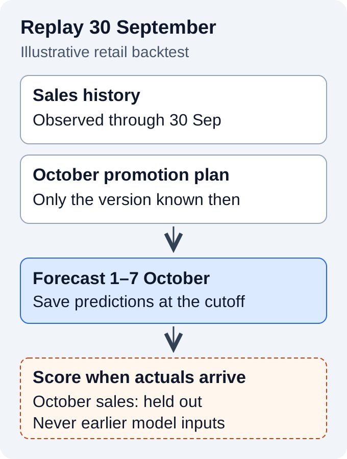
Consider a retailer forecasting daily units sold for 100 established SKUs, seven days ahead. For an illustrative historical run, freeze the data at the end of 30 September and predict 1–7 October. Give every record both an event date and an availability timestamp. A refund posted on 3 October cannot silently revise the input available on 30 September merely because it refers to an earlier sale.
Separate three input roles. Past sales are the target history. Historical stock availability is a possible past-only feature. An October promotion schedule can be a known-future feature only if that exact schedule was recorded before the cutoff. A campaign edited on 2 October belongs to a later forecast.
Keep versioned extracts and record when each field became available. A data engineering engagement should specify that history alongside identifiers, time zones and late-arriving records. Without it, a remarkably accurate backtest may simply be benefiting from information that a real operator would not have had.
Read the limits in time steps, not language tokens
The official Timestral-209M model card lists up to 32,768 historical time steps, 1,024 forecast steps in a single forward pass and 21 output quantiles. It supports univariate or multivariate targets, past-only and known-future covariates, and CPU or GPU inference. For longer horizons, successive forecast blocks feed their medians back into the context. That is a different computation from predicting the entire horizon in one pass.
Sampling frequency therefore changes the operational meaning of the same limit. At 15-minute resolution, 32,768 observations span about 341.3 days and 1,024 future steps span about 10.7 days. At daily resolution, a seven-day forecast uses only seven future steps. These are unit conversions, not recommendations to provide the maximum history. Compare shorter windows where older product behaviour may no longer represent the current catalogue.
The quantiles let an application express uncertainty instead of displaying one deceptively precise number. A 10th-to-90th-percentile band is intended to cover 80% of outcomes when calibrated; its actual coverage must be measured. Also distinguish daily uncertainty from weekly uncertainty: adding seven daily upper quantiles does not generally produce the weekly upper quantile. A replenishment policy needs an explicit treatment of dependence across days.
Define the target carefully before comparing errors. Recorded sales can be zero because demand was absent, stock was unavailable or the feed failed. Preserve those distinctions rather than replacing every missing value with zero. If lost demand is unobserved, call the result a sales forecast and document the limitation before using it to set stock levels.
Check weight licensing before estimating deployment costs
The official inference repository provides standalone code and checkpoint links, with support for loading local files. The reviewed release presents downloadable models, without a preview label; that does not establish a managed API's general-availability status or SLA. The model card currently shows no Hugging Face Inference Provider deployment for the 209M checkpoint.
There are two licenses to track. The repository code uses Apache 2.0, while the model weights' Modified MIT license includes a commercial restriction: rights under that license are unavailable if the company or employer's global consolidated monthly revenue exceeded US$20 million in the preceding month. It also requires attribution and permission notices in copies or substantial portions. Affected organisations need to resolve commercial licensing with Mistral before deployment; the code's license does not remove the weights' terms.
We found no Timestral-specific hosted inference rate in the reviewed public pricing page. Treat that as an unverified hosted price, not a claim that every deployment is free. For a local trial, budget compute, data preparation, monitoring and any applicable commercial agreement. Language-model prices per million tokens are not a suitable substitute for the cost of this numerical workload.
As an illustrative planning calculation, suppose a worker is allocated two hours nightly at an assumed US$0.20 per hour. Thirty nights cost US$12 in allocated compute. This is neither a vendor quote nor measured Timestral performance. Add storage, orchestration and support separately. If that two-hour window must process 100 SKUs across eight evaluation cutoffs, the budget is nine seconds per SKU-cutoff job on average, including overhead. Measure the actual job before choosing a machine.
Build a rolling backtest with a fair baseline
First, choose the decision cadence. For a weekly replenishment meeting, use eight historical weekly cutoffs and a seven-day horizon, with enough earlier history at each cutoff. Reserve a later period for final acceptance after tuning. Write the SKU eligibility rule before looking at results, and retain discontinued or difficult items where they were genuinely part of the decision at the time. Otherwise the evaluation can quietly become a test of surviving bestsellers.
Second, create the same input snapshot for every candidate. Begin with a seasonal-naive baseline that repeats the previous week's corresponding daily sales, plus the team's current forecasting method if one exists. Test Timestral with target history alone, then add eligible covariates. This separates the effect of the model from the effect of giving it better information. Keep calendar alignment, missing-value rules and forecast horizon identical across candidates.
Third, run each cutoff without consulting its future targets. Save model and code revisions, input identifiers, forecast arrays, timing, memory use and failures. Pinning a checkpoint matters when reproducing a disputed forecast months later. The repository's input documentation distinguishes past covariates from known covariates spanning history and horizon; validate those shapes and dates before inference. Do not let a successful function call stand in for a verified data boundary.
Fourth, analyse the paired results by horizon and SKU group. Report promotional versus ordinary periods, intermittent sellers and products with stockouts separately. Compare all models on the same successfully prepared cases, and report excluded or failed cases explicitly. A candidate that looks better only after its hardest jobs disappear from the denominator is not ready for an operational decision.
Score uncertainty as well as the central forecast
For the median forecast, calculate mean absolute error and signed error in units sold. The signed error exposes systematic overprediction or underprediction that an average absolute error hides. Add a scale-aware comparison across products, but keep unit-level results for the buyer who must order inventory. Avoid relying on percentage errors for days with zero sales. State whether aggregation gives every SKU equal weight or weights by volume.
For a quantile q, pinball loss is q times the shortfall when actual sales exceed the predicted quantile, and (1 − q) times the excess when the prediction exceeds actual sales. Consider an invented 90th-percentile prediction of 120 units. An actual value of 140 produces a loss of 0.9 × 20 = 18; an actual value of 100 produces 0.1 × 20 = 2. The asymmetry is intentional. These numbers illustrate the score and are not model outputs.
Count how often actuals fall within the 10th-to-90th-percentile band, and record the band's width. If 72 of 100 observations land inside, empirical coverage is 72%, not the nominal 80%. A wider band may improve coverage while becoming less useful for ordering decisions. Check the tradeoff by horizon and product group, and avoid interpreting one small sample as definitive calibration evidence.
Finally, replay the proposed ordering rule using explicit lead times, opening inventory, pack sizes and shortage or holding-cost assumptions. Separate this policy simulation from forecasting accuracy. A lower error does not automatically reduce inventory cost when ordering constraints dominate. Review the assumptions with the operations owner; simulated savings remain illustrative until a controlled deployment measures actual outcomes.
Connect the result to an inspectable merchant workflow
Daphnis's PA: Product & Collection Sort case study provides a relevant integration context: a Shopify merchant application using sales and inventory signals, RFM algorithms and a self-hosted MegaBeam-Mistral-7B model. It documents merchandising work, not Timestral adoption or demand-forecasting performance. A new forecast should remain a separate, versioned input whose effect on merchant decisions can be inspected.
Start a pilot in shadow mode: generate dated recommendations without issuing purchase orders. Give reviewers the forecast range, data cutoff, stockout flags and fallback result. Set acceptance criteria before the trial, such as performance against the seasonal baseline on agreed SKU groups, tolerable underprediction and completion before the planning deadline. A predictive analytics implementation can turn those criteria into an evaluation and handover brief.
When a forecast eventually feeds an action, keep the boundary explicit. Our guide to separating read, draft and send permissions applies to proposed purchase orders as well as messages. A planner should approve a specific quantity and destination with a known data version. Bring a sample sales extract, promotion-history records and the current ordering rule to the first review; those artifacts will expose the real integration work faster than another leaderboard comparison.